Student's t-test
When I was working with bioinformaticians in drug discovery research I’d often hear scientists performing t-test on their data. Often, it’s mentioned with such terms as p-value, rejecting the null hypothesis and significance. Today, I attended a statistics class and learnt how to do it myself.
There are three kinds of t-tests:
- One-sample t-test
- Two-sample t-test (a.k.a independent t-test)
- Paired t-test
One-sample t-test
The one-sample t-test is the simplest and can be used to compare a sample mean against its population mean. The null hypothesis, H0, here is that the sample mean has no difference compared to the population mean.
For example, supposed a factory makes bookshelves that can withstand 40kg of force. Here, the population mean is 40. They’ve been making bookshelves for decades and all these years the mean is 40.
Recently, the factory employed a new method of manufacturing that’s supposed to increase the strength. The followings are the strengths of a few bookshelves taken at random:
| Sample # | Strength |
|---|---|
| 1 | 39.6 |
| 2 | 40.2 |
| 3 | 40.9 |
| 4 | 40.9 |
| 5 | 41.4 |
| 6 | 39.8 |
| 7 | 39.4 |
| 8 | 41.8 |
| 9 | 43.6 |
Question: does the new manufacturing method produce significant strength difference compared to the historical average?
Answer: Enter one-sample t-test
I won’t go through the equation here, which can be found on wikipedia. Instead, I’d use R to quickly get the result and interpret it.
> strengths = c(39.6, 40.2, 40.9, 40.9, 41.4, 39.8, 39.4, 41.8, 43.6)
> t.test(strengths, mu=40)
One Sample t-test
data: strengths
t = 1.9176, df = 8, p-value = 0.09145
alternative hypothesis: true mean is not equal to 40
95 percent confidence interval:
39.82897 41.85992
sample estimates:
mean of x
40.84444
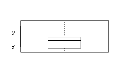
> boxplot(strengths)
> abline(h=40, col="red")
> A commonly accepted p-value cutoff is 0.05. If our sample p-value is ≤ 0.05, we reject the null hypothesis. If our sample p-value is > 0.05, we fail to reject the null hypothesis. Here, our one-sample t-test has a p-value of 0.09, so we fail to reject the null hypothesis. In other words, we fail to find a difference between our sample mean and the population mean, and the new manufacturing method does not produce stronger bookshelves.
The new bookshelf strengths can be visualised using a box plot. The way to read box plots will be saved for another article.
Another example could be human intelligence. We know average IQ among a population is 100. Now, if we have a group of people with the following IQ scores, we can similarly perform a one-sample t-test to find if this group of people are cleverer than the population average:
| Sample # | IQ |
|---|---|
| 1 | 102 |
| 2 | 111 |
| 3 | 108 |
| 4 | 96 |
| 5 | 100 |
| 6 | 104 |
| 7 | 98 |
| 8 | 102 |
| 9 | 116 |
| 10 | 108 |
> iq = c(102, 111, 108, 96, 100, 104, 98, 102, 116, 108)
> t.test(iq, mu=100)
One Sample t-test
data: iq
t = 2.2934, df = 9, p-value = 0.04751
alternative hypothesis: true mean is not equal to 100
95 percent confidence interval:
100.0613 108.9387
sample estimates:
mean of x
104.5
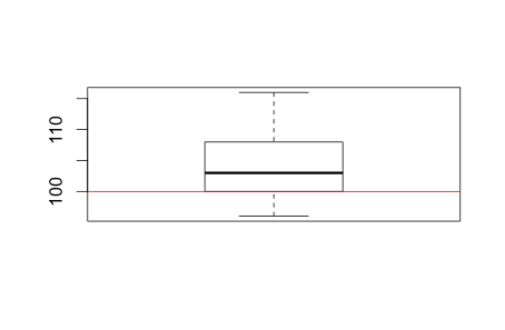
> boxplot(iq)
> abline(h=100, col="red")
>The sample p-value is smaller than 0.05, therefore we reject the null hypothesis that there’s no difference between the sample mean and population mean. In other words, there is a difference. This group is people are really cleverer than the population average. Mensa members, perhaps?
Two-sample t-test
When you have two samples from different populations, two-sample t-test can be used to tell if there’s a difference between the populations. For example, if in your chain of supermarkets you place super-vitamin on normal shelves among other vitamin brands in 10 stores, and in a separate 10 stores you place the same super-vitamin on specially-decorated end-of-aisle shelves. Now you can use two-sample t-test to see if placing super-vitamin on end-of-aisle shelves increases sales.
| Normal | End-of-aisle |
|---|---|
| 22 | 52 |
| 34 | 71 |
| 52 | 76 |
| 62 | 54 |
| 30 | 67 |
| 40 | 83 |
| 64 | 66 |
| 84 | 90 |
| 56 | 77 |
| 59 | 84 |
> normal = c(22, 34, 52, 62, 30, 40, 64, 84, 56, 59)
> aisle = c(52, 71, 76, 54, 67, 83, 66, 90, 77, 84)
> t.test(aisle, normal)
Welch Two Sample t-test
data: aisle and normal
t = 3.0446, df = 15.723, p-value = 0.007849
alternative hypothesis: true difference in means is not equal to 0
95 percent confidence interval:
6.568701 36.831299
sample estimates:
mean of x mean of y
72.0 50.3
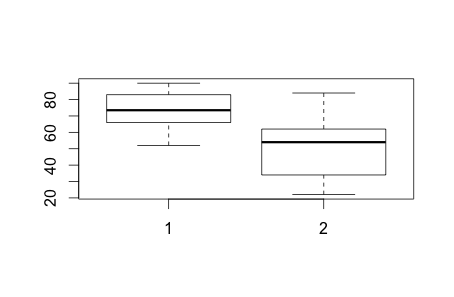
> boxplot(aisle, normal)
> As we can see, the two-sample t-test p-value is much smaller than 0.05, therefore we reject the null hypothesis. In other words, there is a significant difference between the means of normal shelves vs special end-of-aisle shelves.
Paired t-test
Supposed a stock investor wants to find out if there is a significant difference in companies’ P/E ratio between two years. Paired t-test can be used to test the data like so:
| Company | Year1 | Year2 |
|---|---|---|
| 1 | 8.9 | 12.7 |
| 2 | 38.1 | 45.4 |
| 3 | 43.0 | 10.0 |
| 4 | 34.0 | 27.2 |
| 5 | 34.5 | 22.8 |
| 6 | 15.2 | 24.1 |
| 7 | 20.3 | 32.3 |
| 8 | 19.9 | 40.1 |
| 9 | 61.9 | 106.5 |
> year1 <- c(8.9, 38.1, 43, 34, 34.5, 15.2, 20.3, 19.9, 61.9)
> year2 <- c(12.7, 45.4, 10, 27.2, 22.8, 24.1, 32.3, 40.1, 106.5)
> t.test(year1, year2, paired = TRUE)

	Paired t-test

data:  year1 and year2
t = -0.69909, df = 8, p-value = 0.5043
alternative hypothesis: true difference in means is not equal to 0
95 percent confidence interval:
 -21.63607  11.56941
sample estimates:
mean of the differences
              -5.033333

>
The p-value is > 0.05, therefore we failed to reject the null hypothesis. In other words, there is no significant difference between the P/E ratios in the 2 years across the 9 companies. Other uses of paired t-test include tumour size difference before and after drug treatment in the same patient.
It should be noted that the difference between independent and paired t-test is quite subtle. For example, if I want to do A/B testing of a website I have to use one or the other depending on what I’m trying to test. If I want to find out whether women, compared to men, respond more strongly to a webpage, I’d use independent t-test. The two independent populations are women and men and I have to keep my webpage identical. On the other hand suppose I want to test if people click on green buttons more often than red buttons, I would serve an otherwise identical webpage with either a green or a red button randomly to the same population. I’d then use paired t-test to compare the number of times the buttons are clicked on to find their differences.