Correlation analysis and linear regression
Correlation Analysis
Today I learnt correlation analysis. The simplest thing is a table of two variables, income and meat consumption, say. We want to find out how one variable (independent variable, income) correlates with another (dependent variable, meat). First, we want a way to explore and visualise the data to see if they are correlated. A scatter plot is one way to visualise such data.
| Annual income, $,000 | Annual meat consumption, kg |
|---|---|
| 20 | 8 |
| 30 | 20 |
| 100 | 50 |
| 200 | 75 |
| 300 | 78 |
| 500 | 79 |
> income <- c(20, 30, 100, 200, 300, 500)
> meat <- c(8, 20, 50, 75, 78, 79)
> plot(income, meat, xlim = c(0, 600), ylim = c(0, 100))
> cor(income, meat)
[1] 0.8380359
> cor.test(income, meat)

	Pearson's product-moment correlation

data:  income and meat
t = 3.0719, df = 4, p-value = 0.03722
alternative hypothesis: true correlation is not equal to 0
95 percent confidence interval:
 0.08276373 0.98183443
sample estimates:
      cor
0.8380359

> 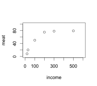
The strength of the correlation can be tested using the cor and cor.test functions in R. The 0.84 returned by cor means 84% of the observed meat consumption can be explained by income. The remaining 16% is not covered by our model. To say a correlation is significant, a value of 0.7 and above must be obtained.
In addition to the correlation strength, we must also check the correlation p-value. The null hypothesis is that there is no relationship between income and meat consumption. A p-value < 0.05 means we reject the null hypothesis. Our p-value of 0.04 does just that. In other words, we reject the null hypothesis and accept that there is a correlation between rising income and rising meat consumption. A possible outcome when doing cor.test is we have strong confidence (low p-value) that there is no correlation (low cor value).
Linear regression
Next, I learnt linear regression. The simplest kind is simply called simple linear regression. It is used to predict how a variable changes (the dependent variable on the y-axis) when another variable changes (the independent variable on the x-axis). An example we used in class is how motor insurance premium (dependent variable) changes with years of driving experience (independent variable) using the following data set.
| Years of driving experience | Motor insurance premium |
|---|---|
| 5 | 64 |
| 2 | 87 |
| 12 | 56 |
| 9 | 71 |
| 15 | 44 |
| 6 | 56 |
| 25 | 42 |
| 16 | 60 |
The following R script produces a scatter plot of the data, fits a regression line and computes the strength of the line.
> exp <- c(5,2,12,9,15,6,25,16)
> prem <- c(64,87,56,71,44,56,42,60)
> plot(exp, prem, xlim=c(0,30), ylim=c(0,100))
> reg <- lm(prem~exp)
> abline(reg, col="red")
> summary(reg)

Call:
lm(formula = prem ~ exp)

Residuals:
     Min       1Q   Median       3Q      Max
-12.0632  -6.7595   0.1349   7.3576  12.7934

Coefficients:
            Estimate Std. Error t value Pr(>|t|)
(Intercept)  77.2784     6.5942  11.719 2.33e-05 ***
exp          -1.5359     0.4992  -3.077   0.0218 *
---
Signif. codes:  0 '***' 0.001 '**' 0.01 '*' 0.05 '.' 0.1 ' ' 1

Residual standard error: 9.776 on 6 degrees of freedom
Multiple R-squared:  0.6121,	Adjusted R-squared:  0.5474
F-statistic: 9.466 on 1 and 6 DF,  p-value: 0.02175

> 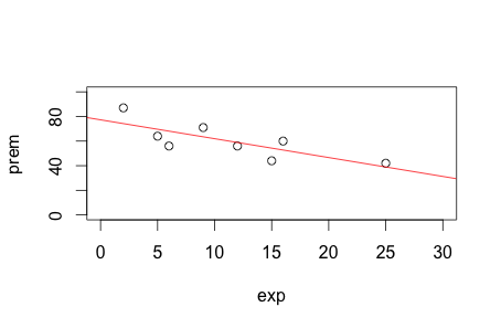
On line 4, reg <- lm(prem~exp) fits a linear model, called reg, to our data and abline simply draws the regression line over a standard scatter plot. A computer program such as R will always be able to fit a line to any model, but whether that model is a good one is a different question. It’s up to us human modellers to answer that question. To do that, we check the adjusted R-squared and p-value. An accepted cutoff for adjusted R-squared is 0.7 but here we only have 0.55. In other words, only 55% of the insurance premium variability can be accounted for by the data. The p-value, though, is low at 0.02 so we reject the null hypothesis.
It is worth asking what the null hypothesis is here. For simple linear regression, H0 is m = 0. The regression line has a general form of y = mx + c. m = 0 implies y = c. In other words, whatever value x (eg, driving experience) takes has no influence on y (ie, motor insurance premium) whatsoever. The regression line becomes a flat line. Rejecting H0 means x influences y.
The summary data of the regression model tells us also how to construct the regression line. From the summary data, we know c = 77.28 and m = -1.54. Therefore, y = 77.28 - 1.54x. So, if you just got your driving licence, expect to pay $77.28, on average. For every year of experience you’ve gained, you pay $1.54 less, again on average. Remember, a regression model is a prediction model and ours only covers 55% of the variation so we can’t be too sure. We can say, though, if you sample a large number of drivers with 10 years driving experience, then their average motor insurance premium is $77.28 - $1.54 * 10 = $61.88.
Life is often more complicated than one variable correlating with another. We often find multiple factors correlating with an observation to varying degrees of strength. Smoking causes cancer, so does alcohol. And if you both drink and smoke which one will do you in? That’s what multiple linear regression tries to answer. Instead of a simple y = mx + c, multiple linear regression has the general form of y = β0x0 + β1x1 + … + βnxn + c + ϵ, where ϵ is the residual error that can’t be explained by the model, c is the y-intercept, and each βi is the coefficient for its corresponding term, xi. The H0 is β0 = β1 = … = βn = 0. The multiple linear regression is best illustrated with an example.
A supermarket chain wants to launch a new energy bar. It sells the energy bar in 34 branches at different prices and varying amount of advertising. We want to find whether it’s low price that increases sales, advertising, both or none.
| Store | Sales | Price | Advertising |
|---|---|---|---|
| 1 | 4141 | 59 | 200 |
| 2 | 3842 | 59 | 200 |
| 3 | 3056 | 59 | 200 |
| 4 | 3519 | 59 | 200 |
| 5 | 4226 | 59 | 400 |
| 6 | 4630 | 59 | 400 |
| 7 | 3507 | 59 | 400 |
| 8 | 3754 | 59 | 400 |
| 9 | 5000 | 59 | 600 |
| 10 | 5120 | 59 | 600 |
| 11 | 4011 | 59 | 600 |
| 12 | 5015 | 59 | 600 |
| 13 | 1916 | 79 | 200 |
| 14 | 675 | 79 | 200 |
| 15 | 3636 | 79 | 200 |
| 16 | 3224 | 79 | 200 |
| 17 | 2295 | 79 | 400 |
| 18 | 2730 | 79 | 400 |
| 19 | 2618 | 79 | 400 |
| 20 | 4421 | 79 | 400 |
| 21 | 4113 | 79 | 600 |
| 22 | 3746 | 79 | 600 |
| 23 | 3532 | 79 | 600 |
| 24 | 3825 | 79 | 600 |
| 25 | 1096 | 99 | 200 |
| 26 | 761 | 99 | 200 |
| 27 | 2088 | 99 | 200 |
| 28 | 820 | 99 | 200 |
| 29 | 2114 | 99 | 400 |
| 30 | 1882 | 99 | 400 |
| 31 | 2159 | 99 | 400 |
| 32 | 1602 | 99 | 400 |
| 33 | 3354 | 99 | 600 |
| 34 | 2927 | 99 | 600 |
> sales <- read.csv("energy_bar.csv")
> reg <- lm(sales$Sales ~ sales$Price + sales$Advertising)
> summary(reg)

Call:
lm(formula = sales$Sales ~ sales$Price + sales$Advertising)

Residuals:
     Min       1Q   Median       3Q      Max
-1680.96  -406.40    53.45   297.48  1342.43

Coefficients:
                   Estimate Std. Error t value Pr(>|t|)
(Intercept)       5837.5208   628.1502   9.293 1.79e-10 ***
sales$Price        -53.2173     6.8522  -7.766 9.20e-09 ***
sales$Advertising    3.6131     0.6852   5.273 9.82e-06 ***
---
Signif. codes:  0 '***' 0.001 '**' 0.01 '*' 0.05 '.' 0.1 ' ' 1

Residual standard error: 638.1 on 31 degrees of freedom
Multiple R-squared:  0.7577,	Adjusted R-squared:  0.7421
F-statistic: 48.48 on 2 and 31 DF,  p-value: 2.863e-10

>
There are a few things to notice here. First, overall p-value is 2.863e-10 and below 0.05 so we reject H0. In other words, price and/or advertising correlate(s) with sales. But which one? We look at the triple stars on the right after sales$Price and sales$Advertising. Reading under the Pr(>|t|) column, the p-value of H0 for βprice=0 is 9.20e-09, way below 0.05. We reject the H0. That means sales$Price has a significant correlation with sales. The same goes for sales$Advertising. Finally, check adjusted R-squared is above 0.7 to ensure our model covers a large portion of sales variation. The significance of the terms can also be obtained using anova:
> anova(reg)
Analysis of Variance Table

Response: sales$Sales
                  Df   Sum Sq  Mean Sq F value    Pr(>F)
sales$Price        1 28153486 28153486  69.152 2.155e-09 ***
sales$Advertising  1 11319245 11319245  27.803 9.822e-06 ***
Residuals         31 12620947   407127
---
Signif. codes:  0 '***' 0.001 '**' 0.01 '*' 0.05 '.' 0.1 ' ' 1
>
Another way to see which independent variable has a correlation is to run step-wise multiple regression. A forward selection adds each independent variable iteratively to see if it’s significant. A significant independent variable is kept. This process goes on under all the independent variables are tested. A backward elimination subtracts terms from the full model. A bidirectional elimination combines both approaches. This process gets tedious very quickly. Luckily, R does it for us in a few lines of code.
> library(MASS)
> step <- stepAIC(reg, direction = "both")
Start:  AIC=442.03
sales$Sales ~ sales$Price + sales$Advertising

                    Df Sum of Sq      RSS    AIC
<none>                           12620947 442.03
- sales$Advertising  1  11319245 23940191 461.80
- sales$Price        1  24556917 37177863 476.77
> step$anova
Stepwise Model Path
Analysis of Deviance Table

Initial Model:
sales$Sales ~ sales$Price + sales$Advertising

Final Model:
sales$Sales ~ sales$Price + sales$Advertising


  Step Df Deviance Resid. Df Resid. Dev      AIC
1                         31   12620947 442.0333
>
Point to note here is we start with an initial model of sales$Sales ~ sales$Price + sales$Advertising and end up with the same final model. Therefore, no term was added or subtracted and both are significantly correlated to sales.
One last interesting thing about our energy bar example is the regression model itself. From the R output, we can construct sales = 3.61 * advertising - 53.22 * price + 5837.52.[1] Take shop 1 for example, we see that the output value of $3,419.54 is pretty close to the real sales value of $4,141. Suppose the company now wants to eliminate advertising because it’s costly. At what price should we sell the energy bar for us to generate the same sales amount? We can just drop the advertising term in our model to get 4141 = 5837.52 - 53.22 * price. It’s trivial to solve the equation to find the new price 31.88.
The following R code shows a different data set following the same multiple linear regression workflow. This time, we want to find which factor correlates to a cigarette’s nicotine content. At the end, we’ll see that a cigarette’s weight and its CO content don’t correlate to its nicotine content. It is the tar that matters.
> cigdata <- read.csv("cigarettes.csv")
> reg <- lm(cigdata$Nicotine.content..mg. ~ cigdata$Tar.content..mg. + cigdata$Weight..g. + cigdata$Carbon.monoxide.content..mg.)
> summary(reg)

Call:
lm(formula = cigdata$Nicotine.content..mg. ~ cigdata$Tar.content..mg. +
    cigdata$Weight..g. + cigdata$Carbon.monoxide.content..mg.)

Residuals:
      Min        1Q    Median        3Q       Max
-0.149411 -0.042048  0.004562  0.048801  0.157792

Coefficients:
                                      Estimate Std. Error t value Pr(>|t|)
(Intercept)                           0.058492   0.195051   0.300    0.767
cigdata$Tar.content..mg.              0.066668   0.010163   6.560  1.7e-06 ***
cigdata$Weight..g.                    0.107696   0.213766   0.504    0.620
cigdata$Carbon.monoxide.content..mg. -0.008062   0.011949  -0.675    0.507
---
Signif. codes:  0 '***' 0.001 '**' 0.01 '*' 0.05 '.' 0.1 ' ' 1

Residual standard error: 0.08002 on 21 degrees of freedom
Multiple R-squared:  0.9553,	Adjusted R-squared:  0.9489
F-statistic: 149.6 on 3 and 21 DF,  p-value: 2.492e-14

> step <- stepAIC(reg, direction = "both")
Start:  AIC=-122.63
cigdata$Nicotine.content..mg. ~ cigdata$Tar.content..mg. + cigdata$Weight..g. +
    cigdata$Carbon.monoxide.content..mg.

                                       Df Sum of Sq     RSS      AIC
- cigdata$Weight..g.                    1  0.001625 0.13609 -124.333
- cigdata$Carbon.monoxide.content..mg.  1  0.002915 0.13738 -124.097
<none>                                              0.13446 -122.633
- cigdata$Tar.content..mg.              1  0.275525 0.40999  -96.763

Step:  AIC=-124.33
cigdata$Nicotine.content..mg. ~ cigdata$Tar.content..mg. + cigdata$Carbon.monoxide.content..mg.

                                       Df Sum of Sq     RSS      AIC
- cigdata$Carbon.monoxide.content..mg.  1  0.003020 0.13911 -125.784
<none>                                              0.13609 -124.333
+ cigdata$Weight..g.                    1  0.001625 0.13446 -122.633
- cigdata$Tar.content..mg.              1  0.292999 0.42909  -97.624

Step:  AIC=-125.78
cigdata$Nicotine.content..mg. ~ cigdata$Tar.content..mg.

                                       Df Sum of Sq     RSS      AIC
<none>                                              0.13911 -125.784
+ cigdata$Carbon.monoxide.content..mg.  1   0.00302 0.13609 -124.333
+ cigdata$Weight..g.                    1   0.00173 0.13738 -124.097
- cigdata$Tar.content..mg.              1   2.86947 3.00858  -50.935
> step$anova
Stepwise Model Path
Analysis of Deviance Table

Initial Model:
cigdata$Nicotine.content..mg. ~ cigdata$Tar.content..mg. + cigdata$Weight..g. +
    cigdata$Carbon.monoxide.content..mg.

Final Model:
cigdata$Nicotine.content..mg. ~ cigdata$Tar.content..mg.


                                    Step Df    Deviance Resid. Df Resid. Dev       AIC
1                                                              21  0.1344637 -122.6334
2                   - cigdata$Weight..g.  1 0.001625209        22  0.1360889 -124.3331
3 - cigdata$Carbon.monoxide.content..mg.  1 0.003020181        23  0.1391091 -125.7843
>
Finally, remember: Correlation is not causation
[1] The equation can be obtained by the following:
> as.formula(
  paste0("sales ~ ", round(coefficients(reg)[1],2), "",
         paste(sprintf(" %+.2f*%s ",
                       coefficients(reg)[-1],
                       names(coefficients(reg)[-1])),
               collapse="")
  )
)
sales ~ 5837.52 - 53.22 * sales$Price + 3.61 * sales$Advertising
Revisions
7 May 2018: Added code for generating linear regression model as formula.
14 March 2017: Original version published.