Using linear regression with non-linear data
Non Linear Data
Real world data often comes in non-linear relationship. Before we can apply linear regression analysis to such data sets, it is necessary to perform linearity transformation first. Population and economic growths are two examples of exponential functions.
The following table shows a familiar example of compound interest.
| Year | Principal |
|---|---|
| 1 | 10000 |
| 2 | 11000 |
| 3 | 12100 |
| 4 | 13310 |
| 5 | 14641 |
| 6 | 16105.1 |
| 7 | 17715.61 |
| 8 | 19487.171 |
| 9 | 21435.8881 |
| 10 | 23579.47691 |
| 11 | 25937.4246 |
| 12 | 28531.16706 |
| 13 | 31384.28377 |
| 14 | 34522.71214 |
| 15 | 37974.98336 |
| 16 | 41772.48169 |
| 17 | 45949.72986 |
| 18 | 50544.70285 |
| 19 | 55599.17313 |
| 20 | 61159.09045 |
| 21 | 67274.99949 |
| 22 | 74002.49944 |
| 23 | 81402.74939 |
| 24 | 89543.02433 |
| 25 | 98497.32676 |
| 26 | 108347.0594 |
| 27 | 119181.7654 |
| 28 | 131099.9419 |
| 29 | 144209.9361 |
| 30 | 158630.9297 |
It’s easy to see principal growth is exponential.
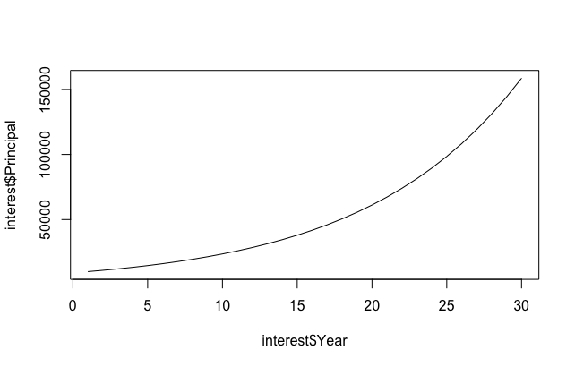
If we attempt to force feed a linear regression model, we’ll get poor results.
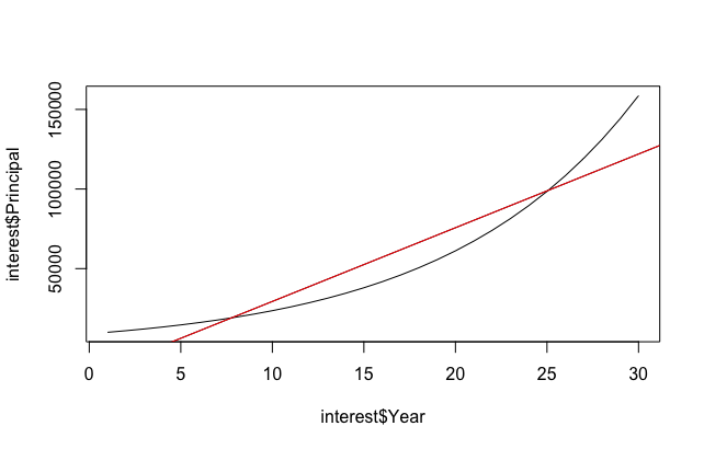
The first step to fix this problem is to understand the nature of the growth of Y with respect to X. Is it a concave function (eg., logarithmic), or is it convex (eg., quadratic, exponential)? In our case, principal growth is exponential, ie., y = ex, so all we need to do is flatten the curve by taking a log.
> interest$LnPrincipal <- sapply(interest$Principal, log)
> interest
   Year Principal LnPrincipal
1     1  10000.00    9.210340
2     2  11000.00    9.305651
3     3  12100.00    9.400961
4     4  13310.00    9.496271
5     5  14641.00    9.591581
6     6  16105.10    9.686891
7     7  17715.61    9.782201
8     8  19487.17    9.877512
9     9  21435.89    9.972822
10   10  23579.48   10.068132
11   11  25937.42   10.163442
12   12  28531.17   10.258752
13   13  31384.28   10.354063
14   14  34522.71   10.449373
15   15  37974.98   10.544683
16   16  41772.48   10.639993
17   17  45949.73   10.735303
18   18  50544.70   10.830613
19   19  55599.17   10.925924
20   20  61159.09   11.021234
21   21  67275.00   11.116544
22   22  74002.50   11.211854
23   23  81402.75   11.307164
24   24  89543.02   11.402475
25   25  98497.33   11.497785
26   26 108347.06   11.593095
27   27 119181.77   11.688405
28   28 131099.94   11.783715
29   29 144209.94   11.879025
30   30 158630.93   11.974336
> plot(interest$Year, interest$LnPrincipal, type='l')
We can verify that ln(Principal) is indeed linear.
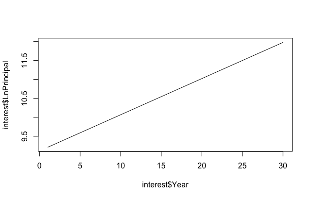
We then run linear regression on ln(Principal). To find out the log values of the principals, we use the predict function.
> reg <- lm(LnPrincipal ~ Year, data=interest)
> predicted <- data.frame(Year=1:35)
> predicted$LnPrincipal <- predict(reg, newdata=predicted)
> predicted
   Year LnPrincipal
1     1    9.210340
2     2    9.305651
3     3    9.400961
4     4    9.496271
5     5    9.591581
6     6    9.686891
7     7    9.782201
8     8    9.877512
9     9    9.972822
10   10   10.068132
11   11   10.163442
12   12   10.258752
13   13   10.354063
14   14   10.449373
15   15   10.544683
16   16   10.639993
17   17   10.735303
18   18   10.830613
19   19   10.925924
20   20   11.021234
21   21   11.116544
22   22   11.211854
23   23   11.307164
24   24   11.402475
25   25   11.497785
26   26   11.593095
27   27   11.688405
28   28   11.783715
29   29   11.879025
30   30   11.974336
31   31   12.069646
32   32   12.164956
33   33   12.260266
34   34   12.355576
35   35   12.450886
>
So far, what we’ve got is the log values of principals. To get the actual dollar values, we only have to raise e to the log values.
> predicted$Principal <- sapply(predicted$LnPrincipal, exp)
> predicted
   Year LnPrincipal Principal
1     1    9.210340  10000.00
2     2    9.305651  11000.00
3     3    9.400961  12100.00
4     4    9.496271  13310.00
5     5    9.591581  14641.00
6     6    9.686891  16105.10
7     7    9.782201  17715.61
8     8    9.877512  19487.17
9     9    9.972822  21435.89
10   10   10.068132  23579.48
11   11   10.163442  25937.42
12   12   10.258752  28531.17
13   13   10.354063  31384.28
14   14   10.449373  34522.71
15   15   10.544683  37974.98
16   16   10.639993  41772.48
17   17   10.735303  45949.73
18   18   10.830613  50544.70
19   19   10.925924  55599.17
20   20   11.021234  61159.09
21   21   11.116544  67275.00
22   22   11.211854  74002.50
23   23   11.307164  81402.75
24   24   11.402475  89543.02
25   25   11.497785  98497.33
26   26   11.593095 108347.06
27   27   11.688405 119181.77
28   28   11.783715 131099.94
29   29   11.879025 144209.94
30   30   11.974336 158630.93
31   31   12.069646 174494.02
32   32   12.164956 191943.42
33   33   12.260266 211137.77
34   34   12.355576 232251.54
35   35   12.450886 255476.70
>
As we can see, the predicted values fit the observed ones remarkably well.