Book summary: Bayesian Statistics the Fun Way
This is a summary and some personal notes of the book by Will Kurt. It is not a book review, but more of notes to my future self. Any error or misinterpretation is mine as I am new to the topic.
Contents
- What is Bayesian statistics
- Bayesian reasoning
- The logic of uncertainty
- Binomial distribution
- Beta distribution
- Conditional probability
- Normal distribution
- Tools for parameter estimation
- Bayesian priors and working with probability distributions
- Parameter estimation with prior probabilities
- Building a Bayesian A/B test
- Bayes factors and posterior odds
- Hypothesis generation
What is Bayesian statistics
Statistics gives us a framework to describe, measure, and infer from data, and there are two broad schools of thought on how to do it.
The Frequentist approach treats the quantity we care about — say, a coin’s true bias — as a fixed but unknown constant, and treats the data as the random thing. Probability here means the long-run frequency of an outcome over infinitely many repetitions of an experiment. You can picture an infinite number of parallel universes, each running the same experiment; the spread of results across them tells us how much to trust an estimate. It answers the question: “how would my procedure (e.g., my way of estimating the bias from n tosses) behave across all those repetitions?”
Bayesian statistics flips this around. The data is what we actually observed and hold fixed; the unknown parameter is treated as uncertain, described by a probability distribution representing our belief. We begin with a prior, combine it with the likelihood of the observed data through conditional probability (Bayes’ theorem), and arrive at a posterior. This lets us change our minds as evidence arrives, judge how much more data we’d need to settle our scepticism, and compare competing hypotheses directly. It complements Frequentist statistics rather than replacing it.
Bayesian reasoning
The book uses the following example as an introduction: one night you woke up and saw a bright saucer-shaped object in the sky. You are sceptical but could this be a UFO?
The steps of Bayesian reasoning are
- Observe data
- Form a hypothesis
- Update beliefs based on the data
Observe data
We can describe the probability of seeing a bright saucer-shaped object in the sky as very low, i.e.,
\[P\left(\textit{bright light, saucer-shaped object in the sky}\right) = \textit{very low}\]The conclusion of ‘very low’ is based on our everyday experience. Therefore, the above can be rephrased using conditional probability by incorporating our prior belief.
\[P\left(\textit{bright light, saucer-shaped object in the sky} \mid \textit{experience on Earth}\right) = \textit{very low}\]It can be abstracted to \(P\left(D \mid X\right) = \textit{very low}\), where D = bright light, saucer-shaped object in the sky, and X = experience on Earth.
Here, we can incorporate more conditions into the prior. Assuming the date is 4th July in the US, where fireworks, drones, and elaborate light displays are common, then \(\textit{X = 4th July USA, experience on Earth}\) and \(P\left(D \mid X\right) = \textit{low}\).
Forming hypotheses
By thinking it’s a UFO, we are in fact forming a hypothesis, H1 = UFO in the sky. Given how unlikely this is, we make more observations and found film crew and wires outside: \(\textit{D' = bright light, saucer-shaped object in the sky, film crew, wires}\) and we then guess people are making films outside, H2.
\[P\left(D' \mid H_2, X\right) >> P\left(D' \mid H_1, X\right)\]When the ratio of the two probabilities:
\[\dfrac{P\left(D' \mid H_2, X\right)}{P\left(D' \mid H_1, X\right)}\]is a large number, say 1,000, it means H2 explains the data 1,000 times better than H1. It’s similar to how we are willing to stake $10 against our friend’s $2 on a hypothesis — a 5:1 ratio — because we rate it at 5-to-1 odds, i.e., five times more likely true than not. It is not an exact thing, but this bet ratio allows us to think how strongly we hold our beliefs.
Using odds to determine probability
Switching to a fresh example, for probabilities that are exhaustive and mutually exclusive, i.e., P(H1) = 1 - P(H2), such as a coin toss, we can use our odds ratio to solve for probabilities.
\[\begin{align*} P\left(H_1\right) &= 5 \times P\left(H_2\right) \\ P\left(H_1\right) &= 5 \times \left(1 - P\left(H_1\right)\right) \\ P\left(H_1\right) &= 5 - 5P\left(H_1\right) \\ 6P\left(H_1\right) &= 5 \\ P\left(H_1\right) &= \dfrac{5}{6} \end{align*}\]In general, \(P\left(H\right) = \dfrac{O \left( H \right)}{1 + O \left( H \right)}\) holds.
The logic of uncertainty
Product rule of probability
To compute the probability of two independent events happening together, we use the product rule of probability. For example, the probability of flipping a tail on a coin AND rolling a six on a die is \(P\left(tail\right) \times P\left(six\right) = \dfrac{1}{2} \times \dfrac{1}{6} = \dfrac{1}{12}\). This is the special case for independent events; in general the product rule is
\[P\left(A \cap B\right) = P\left(A\right) \times P\left(B \mid A\right)\]which we will revisit under conditional probability.
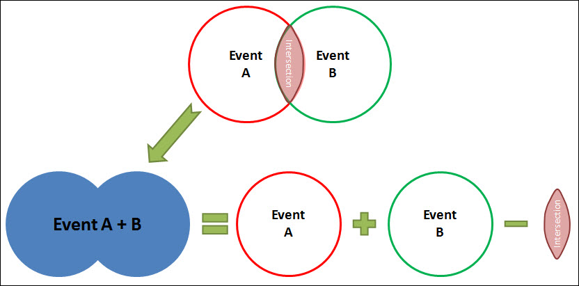
Sum rule of probability
Things get slightly complicated here. We first need to determine if the two events are mutually exclusive.
Sum rule for mutually exclusive events
The probability of getting a tail OR a head is 1. So for any mutually exclusive events, the probability of either is simply their sum.
Sum rule for non-mutually exclusive events
The probability of getting a tail OR tossing a six is \(P\left(tail\right) + P\left(six\right) - P\left(tail, six\right) = \dfrac{1}{2} + \dfrac{1}{6} - \dfrac{1}{2} \times \dfrac{1}{6} = \dfrac{7}{12}\). The last term is to remove double-counting. Visually,
Binomial distribution
The binomial distribution is given by its probability mass function.
\[B(k;n,p) = \binom{n}{k} \times p^k \times \left(1 - p\right)^{n-k}\]By way of illustration, suppose we want the probability of getting exactly two heads in five coin tosses.
\[B\left(2; 5, \dfrac{1}{2}\right) = \binom{5}{2} \times \left(\dfrac{1}{2}\right)^2 \times \left(\dfrac{1}{2}\right)^{5 - 2} = \dfrac{5}{16}\]And suppose now we want the probability of getting at least one head and up to three heads in five tosses, it will be the sum of each k’s probability, i.e.,
\[\sum_{k=1}^{3} \binom{5}{k} \times \left(\dfrac{1}{2}\right)^k \times \left(\dfrac{1}{2}\right)^{5 - k}\]In R, this is pbinom(3, 5, 0.5) - pbinom(0, 5, 0.5), which gives 25/32 ≈ 0.781. pbinom(q, size, prob) returns the cumulative probability \(P\left(X \le q\right)\), so subtracting \(P\left(X \le 0\right)\) from \(P\left(X \le 3\right)\) leaves \(P\left(1 \le X \le 3\right)\).
Beta distribution
Whereas binomial distribution deals with discrete events, such as heads and tails, beta distribution handles continuous range of values. The beta distribution is given by its probability density function.
\[Beta\left(p; \alpha, \beta\right) = \dfrac{p^{\alpha - 1} \times \left(1 - p\right)^{\beta - 1}}{B\left(\alpha, \beta\right)}\]The denominator is the beta function, which is just the numerator integrated across the whole range,
\[B\left(\alpha, \beta\right) = \int_0^1 p^{\alpha - 1} \left(1 - p\right)^{\beta - 1} \, dp\]Dividing by it is what forces the total area under the curve to equal 1, so it acts as a normalising constant. We rarely work it out by hand; R’s dbeta() does the normalising for us. For whole-number parameters it also has the tidy closed form
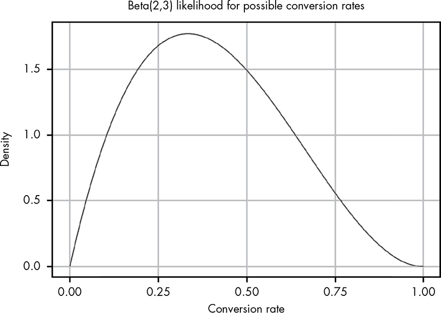
Here, \(\alpha\) is the number of successful events, and \(\beta\) is the number of unsuccessful ones. The book uses an example of a black box that takes in a coin, and it may either eat it up or return two coins. If our first coin in is eaten up, and our second coin is returned with an extra one, we could naively conclude the probability of getting two coins is half. But say we continue to put more coins in to discover the true probability. After 41 coins, we have 14 wins and 27 losses. Now we have two potential probabilities to choose from.
\[P\left(\textit{two coins}\right) = \dfrac{1}{2}\textit{ vs } P\left(\textit{two coins}\right) = \dfrac{14}{41}\]If we think of the event space as \(\textit{two coins}\) and \(\textit{not two coins}\), we can model it using binomial distribution and compare the two probabilities.
\[B\left(14; 41, \dfrac{1}{2}\right) \approx 0.016\textit{ vs } B\left(14; 41, \dfrac{14}{41}\right) \approx 0.130\]This means the assumed probability of \(\dfrac{14}{41}\) explains the observed data 8.125 times better than if we assumed the probability as \(\dfrac{1}{2}\).
So far we have only weighed two candidate probabilities, \(\dfrac{1}{2}\) versus \(\dfrac{14}{41}\), but the true probability could be any value between 0 and 1. This is the continuous bit that the binomial distribution does not handle. The beta distribution treats the probability p itself as a continuous quantity and gives a distribution over every value from 0 to 1. Every extra coin we feed the black box slides us along this curve, shifting where the peak sits between 0 and 1 and tightening the spread as we grow more certain. We can then integrate it from a starting point up to an ending point to find how likely the true probability lies in that range.
If we plot out our observed data in beta distribution we get:
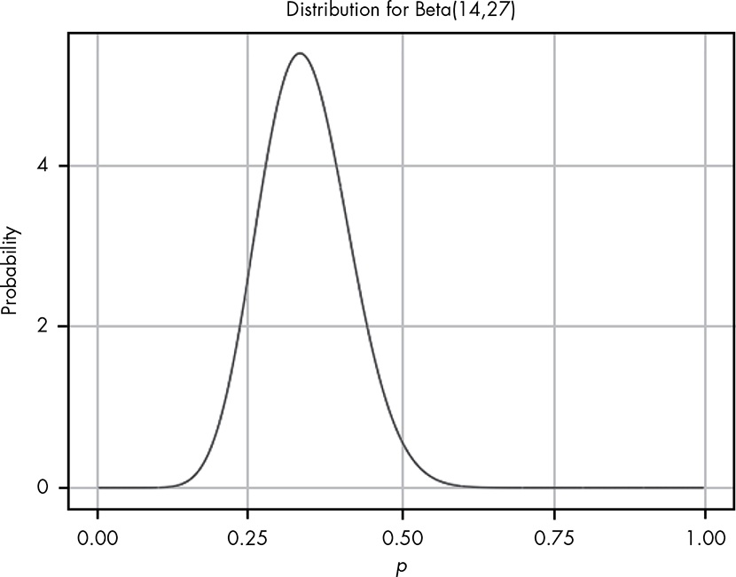
It can be seen that the peak is less than 0.5, meaning there is less than 50% chance we get back two coins based on observed data. So this is a losing game.
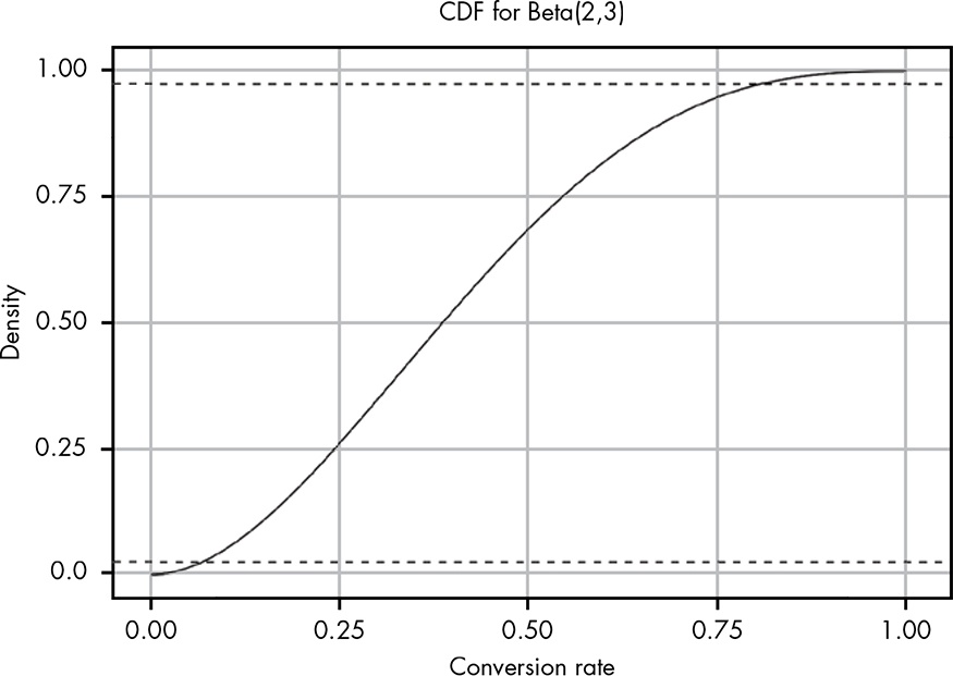
We can find out exactly the chance of getting two coins from the box is less than or equal to 0.5 given the data: integrate(function(p) dbeta(p,14,27), 0, 0.5). This is to integrate the PDF to find the area under curve from 0 to 0.5, and the result is 0.98. In other words, 98% of the area under curve is less than 0.5, as we saw in the plot visually.
In conclusion, beta distribution models the proportion or probability of success. It has a range from 0 to 1. It is possible to model customer sign-up using beta distribution to estimate conversion rate.
Conditional probability
The book gives an example of colour-blindness, a sex-linked problem. The probabilities given are:
\[P\left(\textit{colour blind} \right) = 0.0425 \\ P\left(\textit{colour blind} \mid female\right) = 0.005 \\ P\left(\textit{colour blind} \mid male\right) = 0.08\]Now, assuming we are emailing someone who claims to be colour-blind, what is the chance that they are a male? In other words, \(P\left(male \mid \textit{colour blind}\right) = ?\). It can be found by
\[\begin{align*} P\left(male \mid \textit{colour blind}\right) &= \dfrac{P\left(male\right) \times P\left(\textit{colour blind} \mid male\right)}{P\left(\textit{colour blind}\right)} \\ &= \dfrac{0.5 \times 0.08}{0.0425} \\ &= 0.941 \end{align*}\]Deriving Bayes’ theorem with Lego
The general form of Bayes’ theorem is \(P\left(A \mid B\right) = \dfrac{P\left(A\right)P\left(B \mid A\right)}{P\left(B\right)}\).
Three Lego block pictures reinforced the concept for me for the first time.
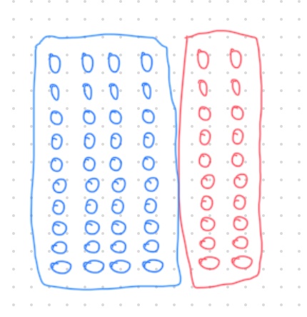
We can see easily \(P\left(blue\right) = \dfrac{40}{60} = \dfrac{2}{3}\). Similarly, \(P\left(red\right) = \dfrac{20}{60} = \dfrac{1}{3}\). Let’s imagine blue as students who passed an exam whereas red represents failing students.
Now, we add a block of 2x3 yellow on top, like so, to represent students who pulled an all-nighter.
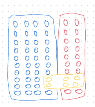
The chance of randomly picking a yellow stud is \(\dfrac{6}{60}\). What is the chance of picking a yellow stud that’s on top of red, i.e., \(P\left(yellow \mid red\right)\)?
We imagine we can split off blue and red.
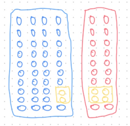
- The area of red is 20.
- Area of yellow is 4.
- Therefore, \(P\left(yellow \mid red\right)\) is \(\dfrac{4}{20}\).
- In other words, of all failing students, one-fifth pulled an all-nighter.
What about \(P\left(red \mid yellow\right)\), the probability of failing the exam, given that one pulled an all-nighter? Visually from the Lego, there are 6 yellow, 4 of which sit on red so the answer is 4/6. Mathematically,
\[\text{numberOfYellowStuds} = P\left(yellow\right) \times \text{totalStuds} = \dfrac{1}{10} \times 60 = 6 \\ \text{numberOfRedStuds} = P\left(red\right) \times \text{totalStuds} = \dfrac{1}{3} \times 60 = 20 \\ \text{numberOfYellowOnRed} = P\left(yellow \mid red\right) \times \text{numberOfRedStuds} = \dfrac{1}{5} \times 20 = 4 \\ \therefore P\left(red \mid yellow\right) = \dfrac{\text{numberOfYellowOnRed}}{\text{numberOfYellowStuds}} = \dfrac{4}{6} = \dfrac{2}{3} \\\]Deriving Bayes’ theorem from this:
\[\begin{align*} P\left(red \mid yellow\right) &= \dfrac{P\left(yellow \mid red\right) \times \text{numberOfRedStuds}}{P\left(yellow\right) \times \text{totalStuds}} \\ &= \dfrac{P\left(yellow \mid red\right) \times P\left(red\right) \times \text{totalStuds}}{P\left(yellow\right) \times \text{totalStuds}} \\ &= \dfrac{P\left(yellow \mid red\right) \times P\left(red\right)}{P\left(yellow\right)} \\ \end{align*} \\ \Rightarrow P\left(A \mid B\right) = \dfrac{P\left(B \mid A\right)P\left(A\right)}{P\left(B\right)}\]The way I think about and remember this is:
- If I touch a stud blindfolded and am told my finger landed on a yellow one, what is the probability mine is a yellow in the red region?
- First, how likely am I to land on the red region in the first instance? That’s my prior, \(P\left(red\right)\).
- How much of the red region could yellow cover? That’s the likelihood, \(P\left( yellow \mid red\right)\).
- Multiplying (2) and (3) is the product rule, and it reads as “how common is red, and of those reds how many have yellow on top?” The answer is the numerator — the joint probability of a stud being yellow-and-on-red, taken as a slice of all studs: \(P\left(red\right) \times P\left(yellow \mid red\right) = \dfrac{1}{3} \times \dfrac{1}{5} = \dfrac{1}{15} = \dfrac{4}{60}\) (the 4 yellow-on-red studs out of 60).
- The denominator, \(P\left(yellow\right)\), is the normaliser — here 6/60, the share of all studs that are yellow. Dividing by it narrows our view from all studs down to the yellow ones alone, turning “yellow-on-red out of all studs” (4/60) into “red out of the yellow studs” (4/6). Closer to 1 means almost every yellow sits on red; closer to 0 means a yellow stud you touch blindly is unlikely to be on red.
- The final answer is called posterior probability.
Normal distribution
The story of this chapter involves six ostensibly identical bomb fuses, five of which have been burnt and their times are known to be 19, 22, 20, 19, and 23. The question is what’s the probability the sixth will be less than 18.
The normal distribution has two parameters, mean (\(\mu\)) and variance (\(\sigma^2\)). In this example, \(\mu = 20.6\) and \(\sigma = 1.82\) (note the change to standard deviation, \(\sigma\) here). This value is the sample standard deviation, with the squared deviations divided by n − 1; the book uses the population value of 1.62 (divided by n), but since the five burnt fuses are really a sample drawn from many, the sample SD is the more fitting choice. Solving the question is essentially finding the area under curve, i.e., \(\int_{-\infty}^{18} N\left(x; \mu = 20.6, \sigma = 1.82\right) \, dx\).
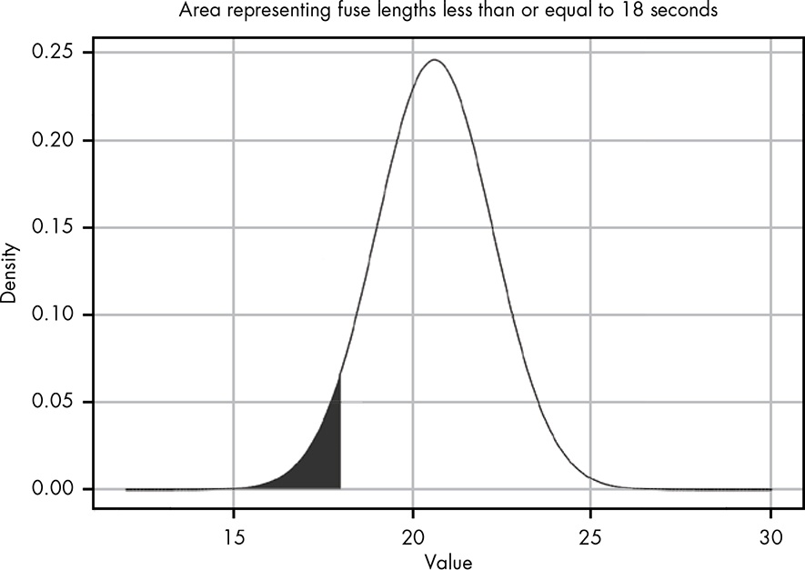
We can’t actually integrate from negative infinity with code but can eyeball the plot and decide 10 to 18 is good enough, since there’s virtually no area below 15 anyway. In R, this can be achieved by integrate(function(x) dnorm(x, mean=20.6, sd=1.82), 10, 18) to get 0.077. That means we are about 92% confident the last fuse will burn for more than 18 seconds, but there’s roughly an 8% chance it will be less.
Tools for parameter estimation
Probability Density Function, PDF
We can find the definite integral of a PDF to get the area under curve. This area represents the probability of a random sample landing in the area. One useful idea is to integrate the lower tail and the upper tail, and compare the two as a ratio to see which is more likely. The way to do this in R is to integrate a d-function, e.g., dnorm(), dbeta().
The famous bell curve is the PDF of the normal distribution.
Cumulative Distribution Function, CDF
The same can be achieved using CDF, which takes in a value and returns the probability of getting that value or lower.
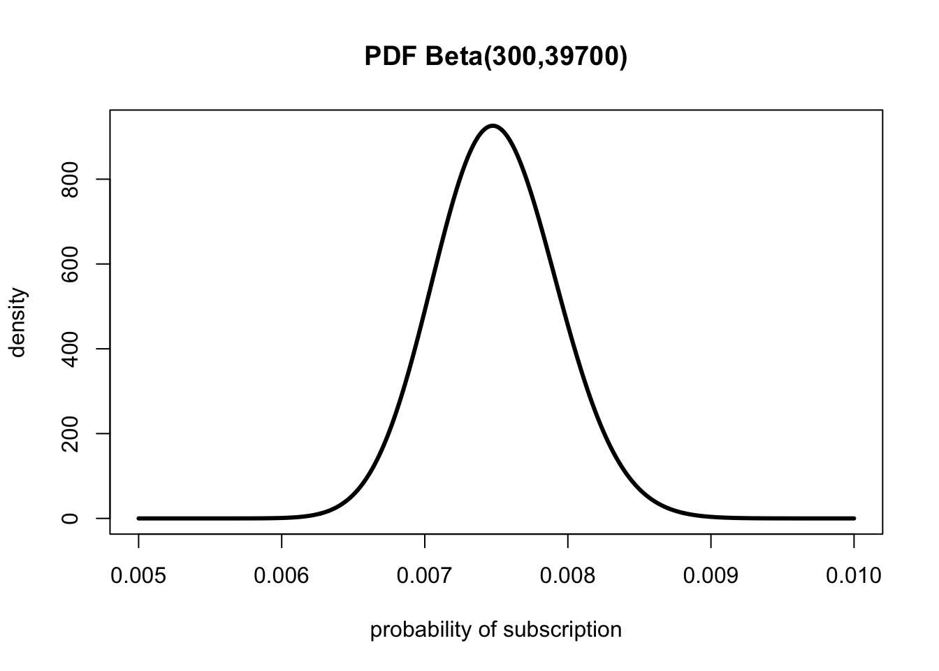
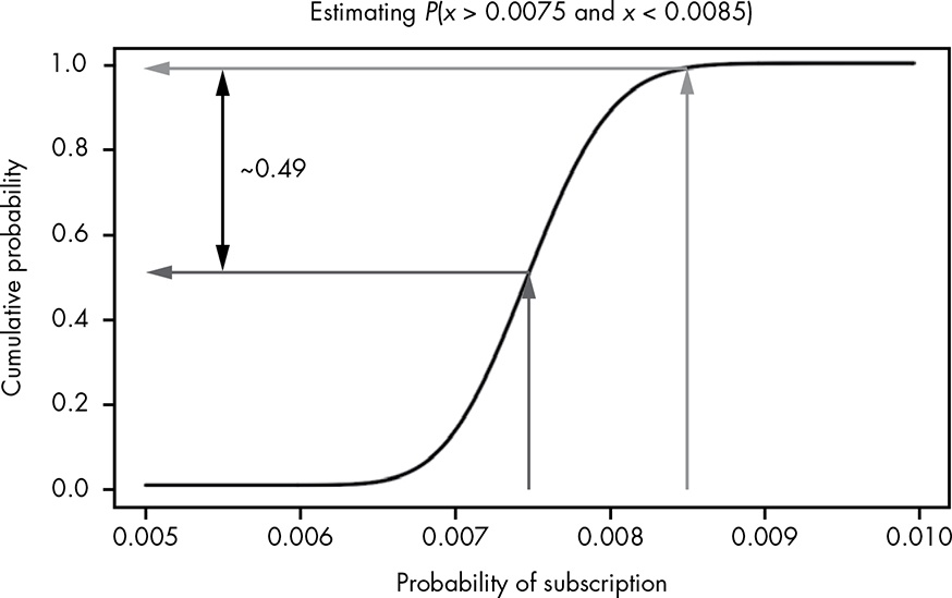
Given the following PDF, we can see its peak sits around 0.0075.
For continuous distributions, finding the median is a lot trickier than the high-school technique of lining numbers up and finding the middle value. CDF makes it easy.
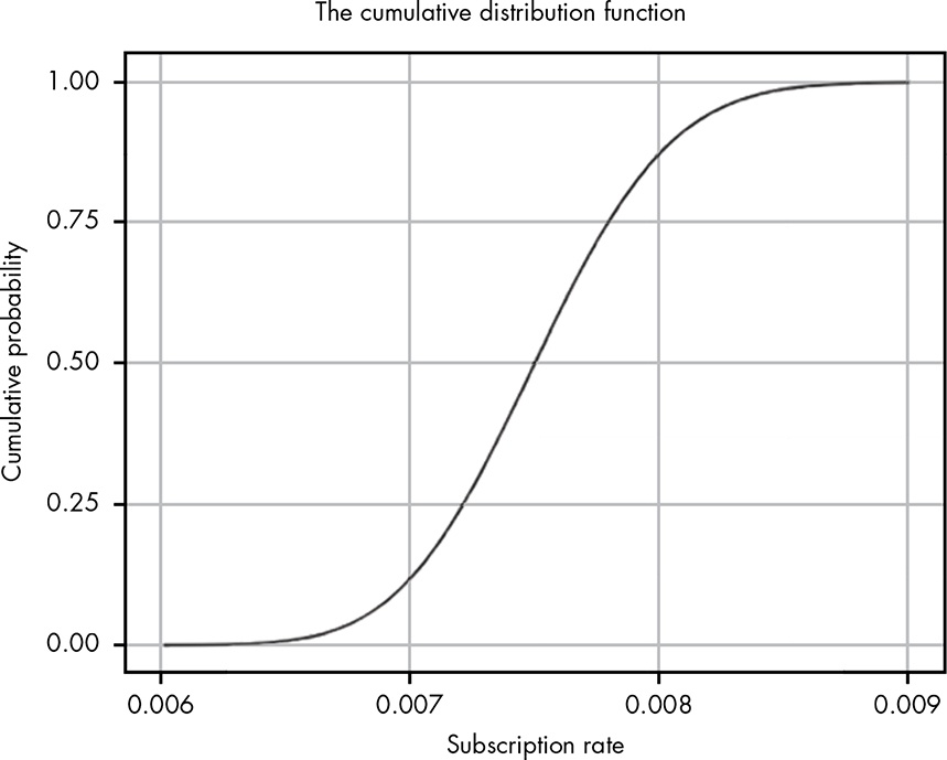
We can also use CDF to visually estimate the probability of the true value being in a certain range. The following example shows the probability of a conversion rate between 0.0075 and 0.0085 is about 0.49.
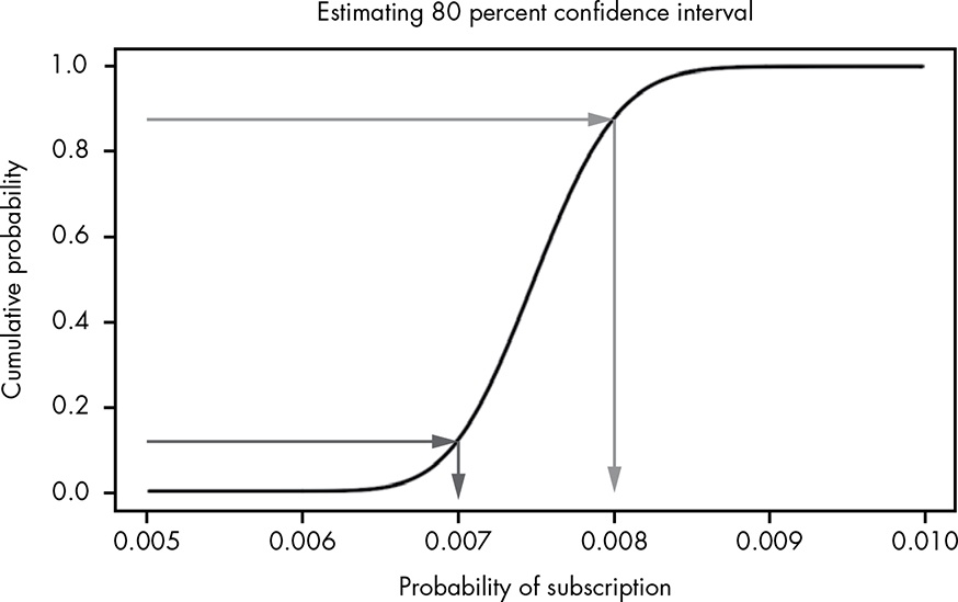
We can also find confidence interval using CDF. Going from y-axis to x-axis, the following estimates an 80% confidence interval between 0.007 and 0.008.
CDFs in R start with p, such as pnorm().
The quantile function
The CDF takes in an x-value and returns its y-value, the cumulative probability of that x-value. When we want to go from y to x mathematically rather than visually as we have done, we need the quantile function. Visually, the quantile function is just the CDF flipped sideway.
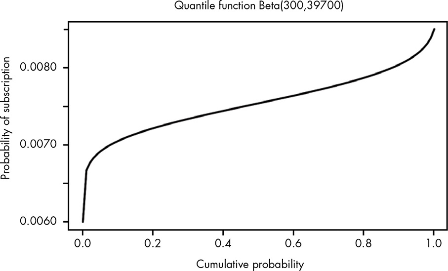
Quantile functions in R are the q functions, such as qnorm(). It takes in a probability (the quantile) and returns the value below which that proportion of the distribution lies. One way to find 95% confidence interval is to compute lower and upper 2.5% quantiles.
We can also run our earlier bomb fuse problem backwards. To be 99% certain of the minimum time the sixth fuse burns, note that being 99% sure it lasts longer than some time t means only 1% of the distribution sits below t — so t is the 1st percentile, qnorm(0.01, mean=20.6, sd=1.82), which gives 16.4 seconds.
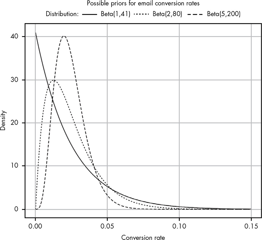
Bayesian priors and working with probability distributions
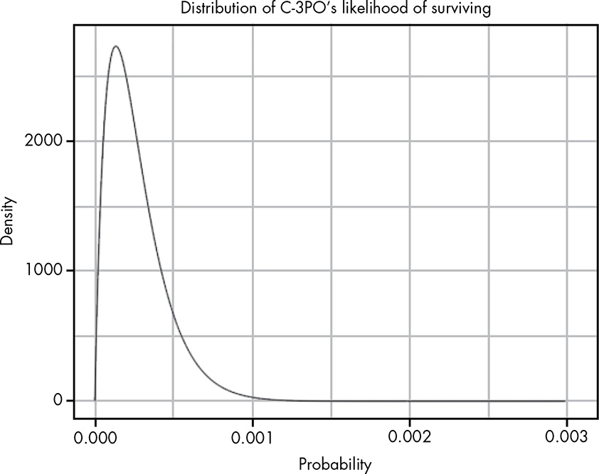
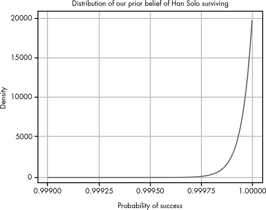
The main idea of this chapter is one can hold an uninformed likelihood of events based on the overall population. Another person may hold a prior belief. The example used is C3PO citing survival statistics of a certain manoeuvre as 3,720 to 1, whilst us the audience of the movie believe it’s near certainty (but not complete certainty, to allow for plot twists) Han Solo will pull it off. C3PO is uninformed, we knew Han Solo is special.
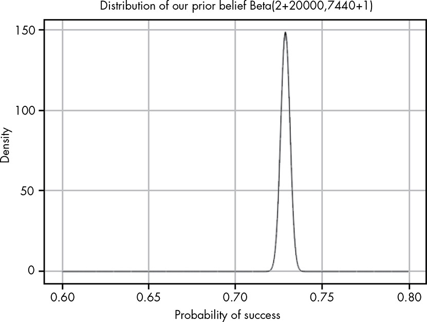
Because this involves proportion of survival amongst all recorded manoeuvres, or probability of survival, beta distribution is appropriate. There is a multitude of ways to express these 3,720-to-1-against odds. Starting with \(Beta\left(1, 3720\right)\) (1 success, 3,720 failures) to \(Beta\left(100, 372000\right)\) and so on. The former is a weaker one, because there is only 1 recorded success, whereas the latter, whilst expressing the same overall ratio, has seen more incidents overall. Doubling to 2 successes and 7,440 failures, C3PO’s likelihood is \(Beta\left(2, 7440\right)\):
Our prior, chosen as 20,000 successes to 1 failure, is \(Beta\left(20000, 1\right)\):
The important concept is we can sum up the two
\[Beta\left(\alpha_{posterior}, \beta_{posterior}\right) = Beta\left(\alpha_{likelihood} + \alpha_{prior}, \beta_{likelihood} + \beta_{prior}\right)\]Our posterior then becomes \(Beta\left(20002, 7441\right)\).
This might be useful for combining general population-level statistics with specific cohort we have beliefs in but lack data.
Parameter estimation with prior probabilities
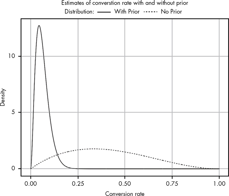
Continuing with \(Beta\left(\alpha_{posterior}, \beta_{posterior}\right) = Beta\left(\alpha_{likelihood} + \alpha_{prior}, \beta_{likelihood} + \beta_{prior}\right)\), the chapter starts with the very first moments of a brand new mailing list that has 2 clicks and 3 no-clicks.
From both the PDF and CDF it can be seen the 95% CI of click-through rate is 0.07 and 0.8. Clearly, the data at this point does not tell us anything useful. What we need to do is borrow some expert experience, i.e., priors. Say, the claimed prior probability is 2.4%. As we have seen, there are infinitely many ways to represent 2.4%. In general, the smaller the total count \(\alpha + \beta\) the weaker the prior. Just as with our non-predictive data, weak priors have a wide spread of possible values so as not to restrain our posterior too much too early. So that’s a good prior to begin with.
The point of adding a weak prior is to restrain our very limited data with some grounding. It’s like saying, between 0.07 and 0.8, here’s a weakly-held assumption that the true rate is around 2.4%. Let’s combine the two and see what happens.
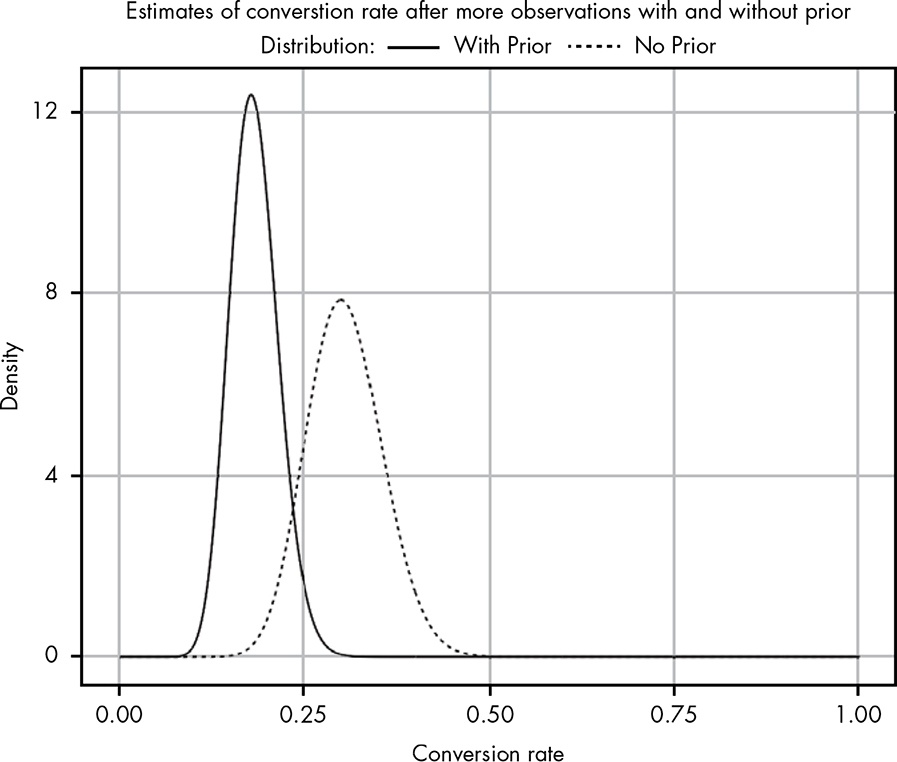
And we gather more and more data to refine our understanding of the true click-through rate.
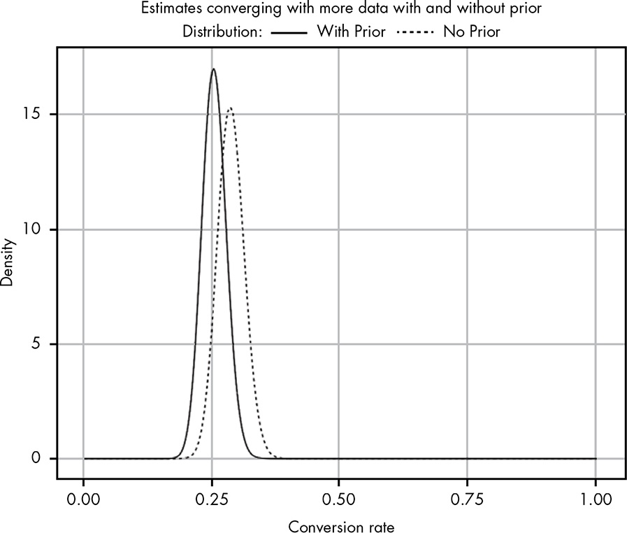
At some point, we will have enough data to come up with our own prior (i.e., we become the new expert).
Building a Bayesian A/B test
This is simply building on and applying \(Beta\left(\alpha_{posterior}, \beta_{posterior}\right) = Beta\left(\alpha_{likelihood} + \alpha_{prior}, \beta_{likelihood} + \beta_{prior}\right)\) to the two variants of an experiment. We apply the same weak prior to the likelihood data collected in the two variants separately. Simple confidence interval comparison and computing the probability that one variant beats the other can be done to check for differences.
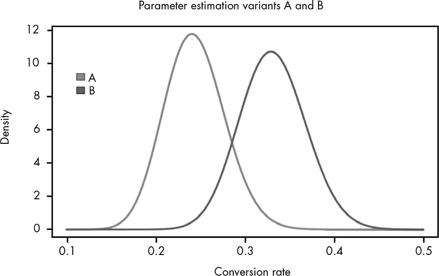
Say, the example mailing list now has two templates and their click-through rate performance is
| Variant | Clicked | Not clicked | Click-through rate |
|---|---|---|---|
| A | 36 | 114 | 0.24 |
| B | 50 | 100 | 0.33 |
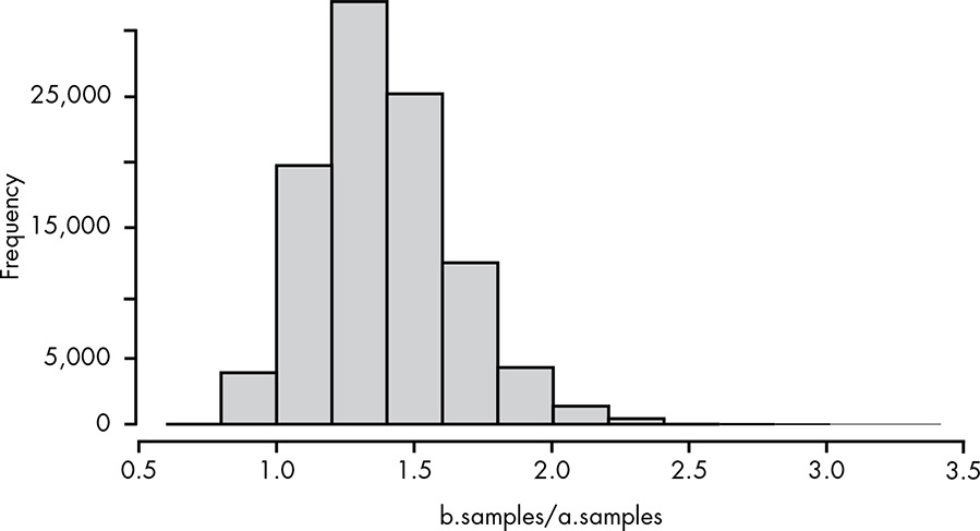
Monte Carlo simulation
The book draws random samples from the posterior distributions of variants A and B (100,000 trials) and counts how often B comes out higher. Each draw from a variant’s posterior Beta is one plausible value of its true click-through rate, so comparing the pairs across 100,000 draws estimates \(P\left(B > A\right)\). This is Monte Carlo simulation — sampling from a distribution we already have.
For the prior we use a weak \(Beta\left(3, 7\right)\) for both variants — a belief that the true click-through rate is around 30%, held lightly (just 10 pseudo-observations) — added to each variant’s clicks and no-clicks via conjugacy.
R code
n.trials <- 100000
prior.a <- 3
prior.b <- 7
a.samples <- rbeta(n.trials, 36+prior.a, 114+prior.b)
b.samples <- rbeta(n.trials, 50+prior.a, 100+prior.b)
p.b_superior <- sum(b.samples > a.samples) / n.trials
We can also plot a histogram of b.samples / a.samples to see the distribution of when B is better or worse than A. It can be seen B is roughly 36% better than A.
Bayes factors and posterior odds
Bayes’ theorem takes this form
\[P\left(H \mid D\right) = \dfrac{P\left(H\right) \times P\left(D \mid H\right)}{P\left(D\right)}\]Quite often we don’t have \(P\left(D\right)\). That leaves us with
\[P\left(H \mid D\right) \propto P\left(H\right) \times P\left(D \mid H\right)\]Posterior odds
This, the posterior odds, allows us to compare two competing hypotheses and see the relative success in explaining the data.
\[\dfrac{P\left(H_{1}\right) \times P\left(D \mid H_{1}\right)}{P\left(H_{2}\right) \times P\left(D \mid H_{2}\right)}\]The posterior odds is further broken down into 2 parts.
Bayes factor
\[\dfrac{P\left(D \mid H_{1}\right)}{P\left(D \mid H_{2}\right)}\]If a friend claims they can predict a fair die 90% of the time, we can set up our hypotheses thus
\[H_{1}: P\left(correct\right) = \dfrac{9}{10} \\ H_{2}: P\left(correct\right) = \dfrac{1}{6}\]It reads, under H1, our friend can truly predict a fair die, getting it right 90% of the time. Under the alternative hypothesis H2, our friend cannot predict and is right only one-sixth of the time. We compute the Bayes factor after our friend guessed 9 out of 10 rolls right.
\[\begin{align*} BF &= \dfrac{P\left(D_{10} \mid H_{1}\right)}{P\left(D_{10} \mid H_{2}\right)} \\ &= \dfrac{\left(\dfrac{9}{10}\right)^9 \times \left(1 - \dfrac{9}{10}\right)^1}{\left(\dfrac{1}{6}\right)^9 \times \left(1 - \dfrac{1}{6}\right)^1} \\ &= 468,517 \end{align*}\]This means the hypothesis that our friend is a psychic explains the observed data 468,517 times better than chance.
Prior odds
\[\dfrac{P\left(H_{1}\right)}{P\left(H_{2}\right)}\]This prior odds of H1 can be written as \(O\left(H_{1}\right)\). If it’s 100, it means without seeing any evidence or data, we are willing to believe H1 explains the data better than H2 by 100 times. This was mentioned earlier in forming hypotheses.
The posterior odds can therefore be rewritten as \(O\left(H_{1}\right) \dfrac{P\left(D \mid H_{1}\right)}{P\left(D \mid H_{2}\right)}\). The following table summarises when we should take notice
| Posterior odds | Strength of evidence |
|---|---|
| 1 to 3 | Interesting, but nothing conclusive |
| 3 to 20 | Looks like we are on to something |
| 20 to 150 | Strong evidence in favour of H1 |
| > 150 | Overwhelming evidence |
Worked example - testing for a loaded die
Suppose in a bag there are 3 six-sided dice, two of them fair and the last one lands on 6 half of the time. We randomly take one out and roll 10 times.
6, 1, 3, 6, 4, 5, 6, 1, 2, 6
We want to find out which die we just rolled. Let’s call H1 be the loaded die, and H2 the regular die.
\[P\left(D \mid H_{1}\right) = \left(\dfrac{1}{2}\right)^4 \times \left(\dfrac{1}{2}\right)^6 = 0.00098\] \[P\left(D \mid H_{2}\right) = \left(\dfrac{1}{6}\right)^4 \times \left(\dfrac{5}{6}\right)^6 = 0.00026\]The ratio of the two likelihoods (the Bayes factor) is 3.77, but only true if there were 2 dice in the bag to equalise H1 and H2. Given there are two fair dice and one loaded one, \(P\left(H_{1}\right) = \dfrac{1}{3}; P\left(H_{2}\right) = \dfrac{2}{3}\), giving \(O\left(H_{1}\right) = \dfrac{1}{2}\). The final posterior odds is actually \(\dfrac{1}{2} \times 3.77 = 1.89\), not supportive of the hypothesis that we just rolled the loaded die.
Worked example - psychic reading dice
When introducing Bayes factor, we encountered a situation when a friend appears to be able to predict dice rolls 90% of the time. If we refuse to believe in psychics, we could set our prior odds to compensate for that.
\[O\left(H_{1}\right) = \dfrac{1}{468,517} \\ posterior = O\left(H_{1}\right) \times \dfrac{P\left(D_{10} \mid H_{1}\right)}{P\left(D_{10} \mid H_{2}\right)} = 1\]But suppose our friend rolls another 5 times and guesses them all right, then even under \(O\left(H_{1}\right)\) our friend is still in psychic territory.
\[posterior = O\left(H_{1}\right) \times \dfrac{P\left(D_{15} \mid H_{1}\right)}{P\left(D_{15} \mid H_{2}\right)} = 4,592\]We could begin to suspect the die is in fact loaded, but must realise we are introducing a new hypothesis. We can proceed to compare H2 and H3 and recompute the posterior. The important point here is we can iterate and introduce new hypotheses and priors, but need to be wary that at some point we will become intransigent and stop listening to data.
Hypothesis generation
The book’s final chapter tells a story of a dispute in a carnival game between the game attendant and a customer. The gist is there is observed data both parties can agree upon, 24 successes and 76 failures. The customer claims a very pessimistic likelihood whilst the attendant a fair chance. Neither explains the data well. The aim is for us to search for the hypothesis that best explains the data.
The way to do it is to parameterise the two hypotheses in Bayes’ factor, and loop over small increments of probabilities from 0 to 1. The best hypothesis is the one that returns the highest Bayes’ factor. In R
dx <- 0.01
hypotheses <- seq(0, 1, by=dx)

bayes.factor <- function(h_top, h_bottom) {
  ((h_top)^24 * (1 - h_top)^76) / ((h_bottom)^24 * (1 - h_bottom)^76)
}

bfs <- bayes.factor(hypotheses, 0.5) # this compares the range of competing customer hypotheses against the attendant's 0.5
plot(hypotheses, bfs, type='l')
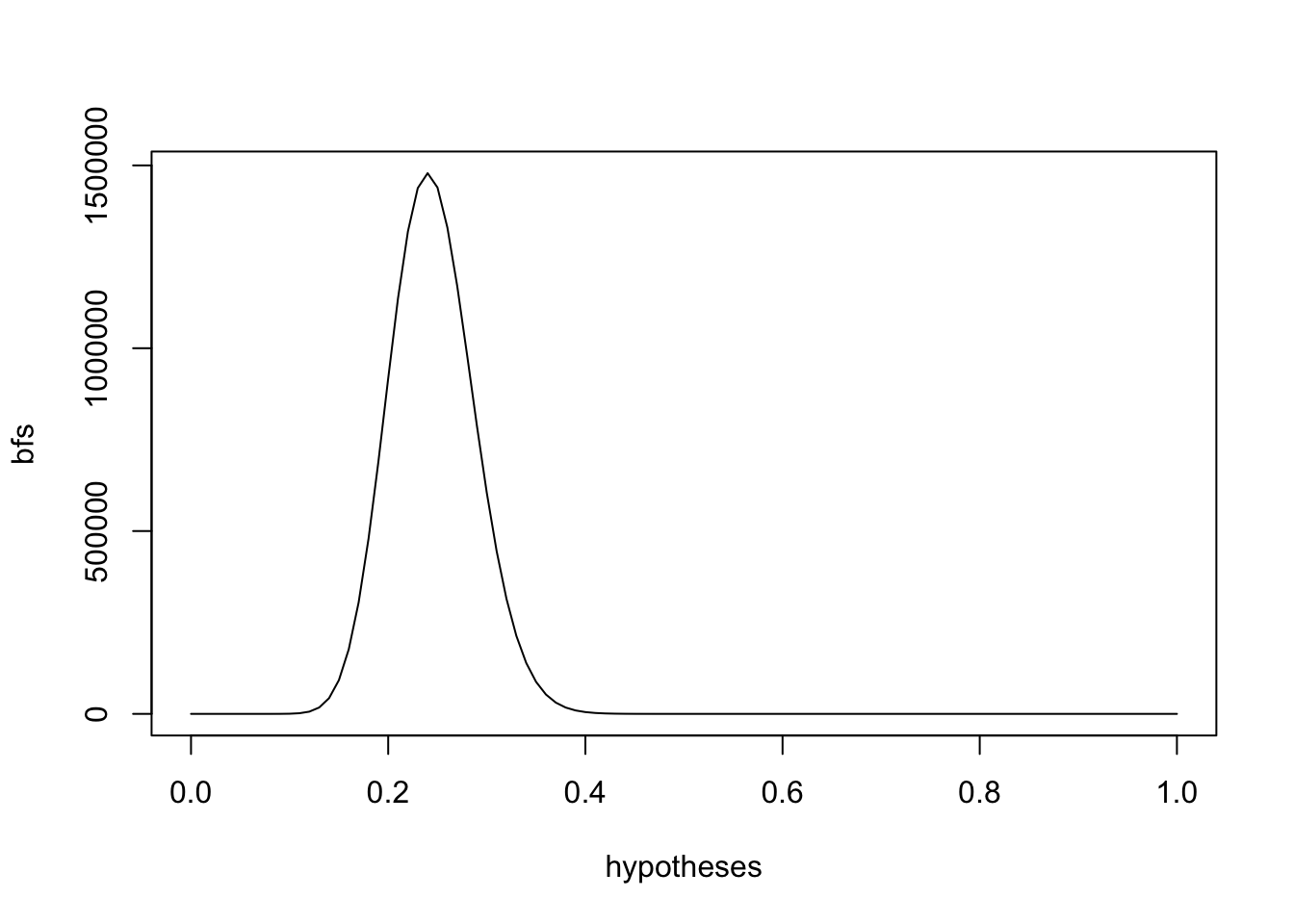
The maximum Bayes’ factor is max(bfs) and the hypothesis at that point is hypotheses[which.max(bfs)]. The book’s example shows 0.24, meaning it’s not fair chance as the attendant claims, nor an overly-pessimistic one alleged by the customer.
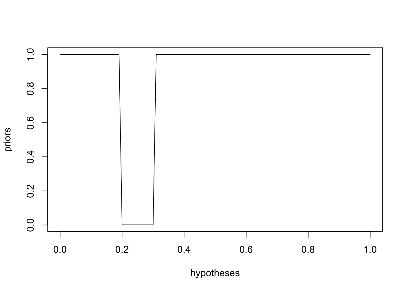
Adding in a prior
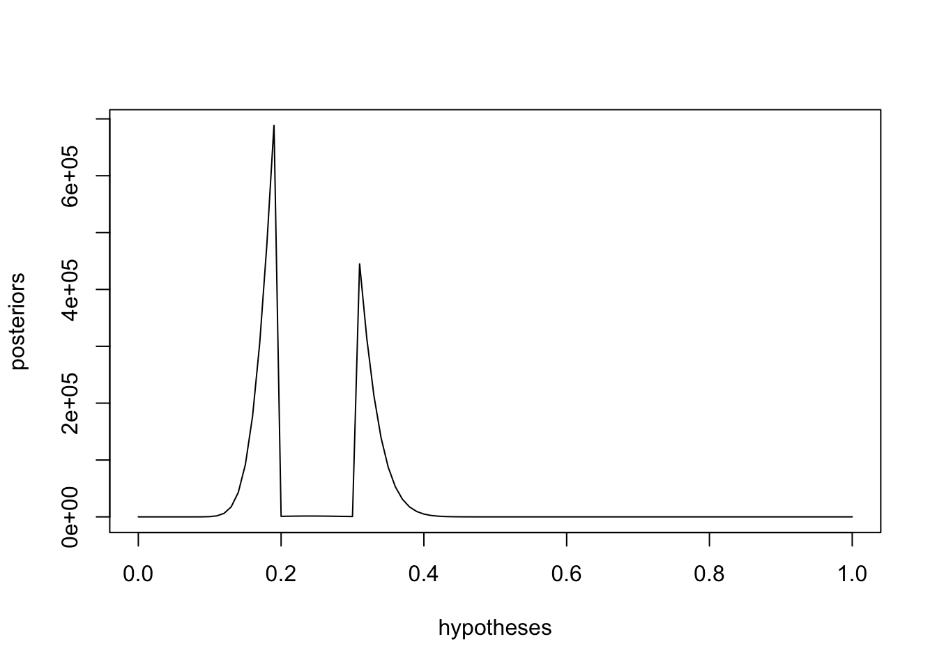
Suppose now a former games manufacturer says the industry never uses a prize rate between 0.2 and 0.3. This could be represented in R as
priors <- ifelse(hypotheses >= 0.2 & hypotheses <= 0.3, 1/1000, 1) # we use 1/1000 here to represent "never"
plot(hypotheses, priors, type='l')
And the full range of posteriors.
posteriors <- priors * bfs
plot(hypotheses, posteriors, type='l')
We can convert the individual posteriors to a distribution.
p.posteriors <- posteriors / sum(posteriors)
plot(hypotheses, p.posteriors, type='l')
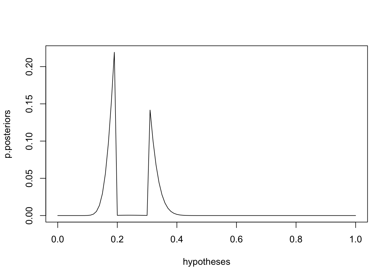
We can now compute the probability that the true prize rate is less than what the attendant claims.
sum(p.posteriors[which(hypotheses < 0.5)])
> 0.9999995
It’s virtually impossible for a fair game (rate 0.5) to have produced the 24-out-of-100 result we observed. The expected value of this distribution is
sum(p.posteriors * hypotheses)
> 0.2402704
Despite the former games manufacturer’s prior, the expected prize rate falls between 0.2 and 0.3. That is different to the most likely estimate that is found by
hypotheses[which.max(p.posteriors)]
> 0.19
Either way we choose, we now have ways to reason with data using Bayes’ theorem.