Linear regression residual visualisations
After running linear regression, it’s important to check for residual. The residual of a linear regression model is the difference between the observed value of the dependent variable y and the fitted value ŷ.
The following table shows how energy bar sales correlate with price and marketing expenditure.
| Store | Sales | Price | Advertising |
|---|---|---|---|
| 1 | 4141 | 59 | 200 |
| 2 | 3842 | 59 | 200 |
| 3 | 3056 | 59 | 200 |
| 4 | 3519 | 59 | 200 |
| 5 | 4226 | 59 | 400 |
| 6 | 4630 | 59 | 400 |
| 7 | 3507 | 59 | 400 |
| 8 | 3754 | 59 | 400 |
| 9 | 5000 | 59 | 600 |
| 10 | 5120 | 59 | 600 |
| 11 | 4011 | 59 | 600 |
| 12 | 5015 | 59 | 600 |
| 13 | 1916 | 79 | 200 |
| 14 | 675 | 79 | 200 |
| 15 | 3636 | 79 | 200 |
| 16 | 3224 | 79 | 200 |
| 17 | 2295 | 79 | 400 |
| 18 | 2730 | 79 | 400 |
| 19 | 2618 | 79 | 400 |
| 20 | 4421 | 79 | 400 |
| 21 | 4113 | 79 | 600 |
| 22 | 3746 | 79 | 600 |
| 23 | 3532 | 79 | 600 |
| 24 | 3825 | 79 | 600 |
| 25 | 1096 | 99 | 200 |
| 26 | 761 | 99 | 200 |
| 27 | 2088 | 99 | 200 |
| 28 | 820 | 99 | 200 |
| 29 | 2114 | 99 | 400 |
| 30 | 1882 | 99 | 400 |
| 31 | 2159 | 99 | 400 |
| 32 | 1602 | 99 | 400 |
| 33 | 3354 | 99 | 600 |
| 34 | 2927 | 99 | 600 |
We then build a linear regression model, reg.
> sales <- read.csv("energy_bar.csv")
> reg <- lm(sales$Sales ~ sales$Price + sales$Advertising)
To plot reg’s residual:
> res <- resid(reg)
> plot(sales$Sales, res)
> abline(0,0)
> 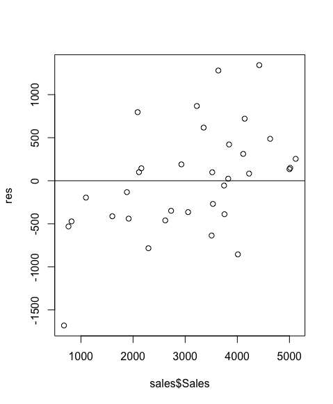
Recall that in linear regression, we’re fitting a straight line to observed values. Some observed values will be underestimated (y > ŷ); some overestimated (y < ŷ); and others right smack on the line (y = ŷ). If the fitted line is a good estimator, then the under- and over-estimations should be random and cancel out each other, on average. This is what is shown in the residual plot above, showing the residual values dancing around the zero line.
Any pattern on the residual plot indicates a systemic error in the model. It could be outliers. Sometimes, data may need to be manually cleaned up. Alternatively, the data set may not in fact be linear. In which case, linearity transformation may be required to flatten a concave or convex function. But the main point is that residual patterns always require investigation.